Tutorials¶

In this section of the tutorial, we provide a number of fairly basic tutorials, covering the usage of various algorithms, operators, and representations within Wallace. All of the tutorials assume that the reader has a basic knowledge of evolutionary algorithms, and that they have read the Basics section of this documentation.

Getting Started¶

Installing IJulia.
Installing Pandas and matplotlib.

Simple Genetic Algorithms and Max Ones¶

In this tutorial, we will be using Wallace to implement a simple Genetic Algorithm to solve the benchmark Max Ones optimisation problem, in which the object is to maximise the number of ones in a fixed-length binary string. This problem is trivial for humans, of course, but proves to be a little trickier for “blind” evolutionary algorithms.

Getting started¶

Once you have Wallace installed on your machine, create a new Julia file for this tutorial, named tut1.jl, or whatever you wish. At the top of this file, don’t forget to make Wallace available via using Wallace.

For the rest of this tutorial, and all the other tutorials, you will now be writing to this (or another) Julia script file, which can be executed from the command line by simply calling:

$ julia tut1.jl

You may find it useful to keep the Julia REPL in another tab, in order to allow you to quickly navigate the Wallace documentation via Julia’s help command. Once in the Julia REPL, if you type ? into the command prompt, the REPL will be switched into help mode. When in this mode, you may enter the name of a particular component, method, type, or Julia function for which you wish to view the documentation.

help> mutation.bit_flip

  Performs bit-flip mutation on a fixed or variable length chromosome of binary
  digits, by flipping 1s to 0s and 0s to 1s at each point within the chromosome
  with a given probability, equal to the mutation rate.

  **Parameters:**

  * `stage::AbstractString`, the name of the developmental stage that this
    operator should be applied to. Defaults to the genotype if no stage is
    specified.
  * `rate::Float`, the probability of a bit flip at any given index.
    Defaults to 0.01 if no rate is provided.

Tip: Don’t forget, in order to view the documentation for Wallace, you must first make Wallace available to Julia by calling ``using Wallace``.

Creating a skeleton for our algorithm specification¶

All algorithm instances within Wallace are first outlined by providing details of the exact configuration to the appropriate algorithm constructor. In this case, as we wish to a Simple GA to solve the problem, we make use of the algorithm.simple_genetic constructor.

Unlike the constructor for algorithm.SimpleGenetic, the underlying type used to implement the simple GA, algorithm.simple_genetic is used to produce a specification of an algorithm, which is then synthesised into an executable instance using the compose! method.

Below is a skeleton for a simple GA definition. The block following the closing parentheses is used to implement the domain-specific language of Wallace, allowing a provided algorithm specification, alg, to be manipulated and completed.

alg = algorithm.simple_genetic() do alg

end

Once we’ve finished filling out the skeleton above, which we will proceed to do over the next few parts of this tutorial, we can compose the algorithm and run it via the following code:

executable = compose!(alg)
run!(executable)

Performance tip: Wrap inside function; don’t use globals.

Specifying the components of our algorithm¶

Now we have our skeleton in place, let’s proceed to specify each of the components of our algorithm. Before we can do this, however, we need to know what the components of our particular algorithm are. In order to find out this information, we can make use of the help function within the Julia REPL (or Juno) to view the information about our algorithm:

julia> using Wallace
help> algorithm.simple_genetic

  DESCRIPTION OF THE SIMPLE GENETIC ALGORITHM

  Properties:

  * evaluator, the evaluator used to compute objective function values for
    the candidate solutions.
  * replacement, the replacement scheme used to determine the membership of a
    deme at each generation, from its existing members and their offspring.
    Defaults to ``replacement.generational`` if none is specified.
  * termination, a dictionary of termination conditions for this algorithm,
    specified as ``criterion`` instances, indexed by their names.
  * population, a specification of the population used by this algorithm,
    detailing its size, demes, species, etc.
  * loggers, a list of loggers that should be attached to this algorithm to log
    various data. Provided as ``logger`` specifications.

Armed with this information, we can now delve deeper into the domain specific language, querying the help function about the types used by each of the properties of our algorithm, such as population, replacement, logger, and so on.

Setting up the population¶

To begin with, let’s specify the population used by our algorithm. For this problem, a simple population, with a single deme and species, specified using population.simple, will suffice. Using the help function, we can find the necessary properties to set up our population.

After specifying the size of our population, the skeleton for our population specification should look similar to the one given below (where the ellipsis will be replaced by species and breeder specifications later on).

alg.population = population.simple() do pop
  pop.size = 100
  pop.species = ...
  pop.breeder = ...
end

Specifying the species¶

In order to complete our population specification, let us next move onto specifying the species to which all of its members belong. Again, for the purposes of this problem, where the search only requires one form of representation, namely the bit-string, the simple species model, species.simple, will suffice.

After performing a help query to learn the properties of species.simple, we will learn that there are only two properties that need to be provided; fitness, specifying the fitness scheme used to transform objective function values returned by the evaluator into fitness values, and representation, used to describe the representation used to model candidate solutions to the problem.

pop.species = species.simple() do sp
  sp.fitness = ...
  sp.representation = ...
end

Designating a fitness scheme¶

First, let us outline the fitness scheme that will be used. You may notice from the documentation for species.simple, that if no fitness scheme is supplied, the species will default to using a scalar fitness scheme, fitness.scalar, where the fitness function returns floating points that are to be maximised.

For our problem, however, we really want fitness values to be represented by integers, rather than performing an unnecessary conversion to a floating point number. A scalar fitness shall still suffice though, so we can provide our species with the following fitness scheme definition:

sp.fitness = fitness.scalar() do f
  f.of = Int
  f.maximise = True
end

Alternatively, as shown in the documentation, we may also elect to specify our fitness.scalar in a number of different ways. We can achieve the same effect in fewer lines of code using the code below, but in the process we possibly trade-off a smaller amount of readability for those less acquainted with Wallace.

sp.fitness = fitness.scalar(Int)

Detailing the problem representation¶

With a fitness scheme now in place, we need only provide a specification of the representation used by candidate solutions within the population. For our particular problem we want to use the bit vector representation, implemented by representation.bit_vector, where solutions take the form of a fixed-length vector of boolean values (representing bits).

Reading the documentation for the representation.bit_vector, we learn that this representation has only a single parameter, namely its length, given by the length property.

For this tutorial, let us create a bit vector of length 100, to begin with. We may do so using either of the definitions given below.

sp.representation = representation.bit_vector() do rep
  rep.length = 100
end

sp.representation = representation.bit_vector(100)

Specifying the breeding operations¶

Now we have a complete species specification, the only thing remaining in our population specification is to provide a description of the breeding process it uses.

Again, we will make use of Wallace’s simplest breeder, breeder.simple, which implements breeding as a process of selection, followed by crossover, and finishing with mutation, with each stage performed by a single operator. Reading the documentation for breeder.simple, we end up with the following skeleton specification:

pop.breeder = breeder.simple() do br
  br.selection = ...
  br.crossover = ...
  br.mutation = ...
end

Selection¶

For the purposes of this tutorial, we will use the simple, but rather effective method of tournament selection as our method of choice, implemented by selection.tournament. After reading the documentation, we can quickly specify a tournament selection via the following:

br.selection = selection.tournament(2)

Where 2 is the size of the tournament.

Crossover¶

As our crossover method, we will use a simple one-point crossover, which accepts two parent genomes are supplied to the operator, following which a random point common to the two genomes is selected, each genome is split into two parts about this point, and finally two new genomes are formed by combining the first and second parts of opposite parents. This method of crossover is implemented by the crossover.one_point operator.

As the only parameter for one point crossover is the crossover rate, which determines the probability that a given pair of chromosomes will be subject to the crossover process, rather than being left alone, we can specify our operator using the following syntax:

br.crossover = crossover.one_point(0.5)

Where 0.5 is the crossover rate.

Mutation¶

Given our use of the bit vector representation, we make use of the most naturally fitting mutation operator, bit flip mutation, implemented by mutation.bit_flip. Bit-flip mutation works by iterating across a provided chromosome and applying a bit-flip at each gene according to some probability, given by the mutation rate.

As with one point crossover, bit flip mutation only accepts a single parameter, the mutation rate. As such, we can concisely specify this operator via the following:

br.mutation = mutation.bit_flip(0.05)

Where 0.05 is the per-gene mutation rate, or the probability that the value of a given gene will be flipped.

Adding an evaluator¶

Next, we will provide our algorithm with an evaluator, responsible for computing the objective function values for provided candidate solutions. For this problem, the simple evaluator, evaluator.simple will suffice. Unlike other components within Wallace, where the block following the method call is used to specify its properties, for the simple evaluator, this block is used to implement the objective function.

The supplied objective function should accept two arguments, the fitness scheme, and the chromosome for the candidate solution, respectively. Once an objective function for the candidate has been computed, a partial fitness value for the individual should be computed from that value and returned. In order to compute the fitness value, we pass the objective value to the assign method, preceded by the fitness scheme.

Since the objective is measured by the number of 1s in a provided bit vector, we can quickly compute the objective value using Julia’s sum function.

Putting together all of the above, we should end up with an evaluator that looks something like the one below.

alg.evaluator = evaluator.simple() do scheme, genome
  assign(scheme, sum(genome))
end

If you query the documentation for the simple evaluator, you may notice it also has two optional keyword parameters. threads is used to specify the number of threads that the evaluation should be split across; leave this for now. The stage parameter is used to specify the name of which of an individual’s developmental stages should be supplied to the evaluator to perform the evaluation; where no value is given, this parameter defaults to using the genotype.

Adding the termination conditions¶

We now have a near complete algorithm specification. The only task remaining is to provide a set of termination conditions, else our algorithm won’t terminate unless the program is forcibly closed by the user.

In order to add a termination condition to our algorithm, we add an named entry into its termination dictionary. We implement each of our mutually inclusive termination conditions using instances of the criterion type. In order to find a list of available criteria, perform a look-up using Julia’s help function on the criterion type.

For this problem, we will simply add a generation limit, which will terminate the algorithm once a given number of generations have passed (where the initialisation phase is not counted as a generation). We can do this using the criterion.generations criterion, as shown below:

alg.termination["generations"] = criterion.generations(1000)

Where 1000 refers to the generation limit.

Running the algorithm and analysing the results¶

Having followed the steps above, you should now have a complete algorithm specification that we can use to solve our problem. Your code should look something similar to that given below:

using Wallace

def = algorithm.genetic() do alg
  alg.population = population.simple() do pop
    pop.size = 100

    pop.species = species.simple() do sp
      sp.fitness = fitness.scalar(Int)
      sp.representation = representation.bit_vector(100)
    end

    pop.breeder = breeder.simple() do br
      br.selection = selection.tournament(2)
      br.mutation = mutation.bit_flip(0.05)
      br.crossover = crossover.one_point(0.5)
    end
  end

  alg.evaluator = evaluator.simple() do scheme, genome
    assign(scheme, sum(genome))
  end

  alg.termination["generations"] = criterion.generations(1000)
end

executable = compose!(alg)
run!(executable)

Give the code a run a few times, using run!, and see what kind of results you can attain using the parameters settings we provided above. You might be disappointed by the end-result of the algorithm, but don’t worry, we’ve given you sub-optimal parameters on purpose.

Can you figure out a better set of parameters, which converge on the global optimum faster? Once you’ve managed that, you might want to try experimenting with other compatible selection and crossover methods, or maybe increasing the difficult of the problem.

Performing search diagnostics with logging and visualisation¶

Currently integrating EvoAnalyser.py into Wallace.

Adding parallel evaluation and breeding¶

So far we have been running (quite intensively) the algorithm on a single thread, but the rest of our available hyper-threads and cores are left doing nothing. In order to maximise our CPU usage, and to maximise the performance of our algorithm, we can use a multi-threaded configuration of our breeder and evaluation to split their respective processes across multiple threads.

Enabling multi-threading within our algorithm is as simply as specifying the number of threads that we wish to split the problem across in our evaluator and breeder definitions. In both cases, the number of threads is specified by the threads parameter, which is accepted as a keyword by the evaluator.simple evaluator.

Try scaling up the difficulty of the problem by increasing the size of the bit vector, then compare the performance of the single-threaded and multi-threaded configurations of the algorithm using Julia’s @time macro, as shown below.

single = algorithm.genetic() do alg
  ...
end

multi = algorithm.genetic() do alg
  ...
end

exec_s = compose!(single)
exec_m = compose!(multi)

run!(exec_s)
run!(exec_m)

@time run!(exec_s)
@time run!(exec_m)

Note, that due to the nature of Julia’s JIT (just-in-time) compiler, the algorithms run faster after they have been run at least once. This difference may be smaller in the future, where each composed algorithm is immediately pre-compiled, prior to being used by ``run!``.

You may also find that performance is slightly improved by running the above code within a function, rather than letting the algorithms become global variables. A few (excellent) tips on improving the performance of general Julia code can be found at: http://docs.julialang.org/en/latest/manual/performance-tips/.

Floating Point Vectors and Numerical Optimisation¶

Building on the previous tutorial, in this tutorial we shall be using simple Genetic Algorithms once again, this time to minimise a series of numerical optimisation benchmark functions. In order to determine the minima of these functions, we make use of the floating point vector representation, used to represent fixed-length real-valued vectors.

Problem¶

Benchmark	Equation	Minimum	Search Domain
Sphere	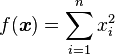$sphere$	$min_sphere$	$dom_sphere$
Rastrigin	$rastrigin$	$min_rastrigin$	$dom_rastrigin$
Rosenbrock	$rosenbrock$	$min_rosenbrock$	$dom_rosenbrock$

Skeleton¶

Rather than declaring our algorithm at the top-level in this tutorial, we will instead write a function which returns a version of our algorithm, tailored to the specifics of one of the benchmarks above. The skeleton of our function should look something like the one given below.

function tutorial_two(size::Int, min::Float, max::Float)
  definition = algorithm.simple_ga() do
    ...
  end
  compose!(definition)
end

Where size::Int is used to specify the number of dimensions, min::Float is used to specify the minimum value that a dimension may take (which is assumed to be equal for all dimensions), and similarly, max::Float specifies the maximum value that a dimension may assume.

Setup¶

For this problem we will be using a near-identical general setup to the one we used in the previous tutorial, given below.

Component	Setting
Population	Simple (single deme)
Breeder	Simple (i.e. selection, crossover, mutation)
Species	Simple (single representation)
Fitness Schema	Scalar (float, minimisation)
Representation	Float vector (length tailored to function)

Fitness Schema¶

As the objective for each of these benchmarks is to find the global minimum value for the function within the bounds of the search domain, our fitness schema should minimise a floating point value, representing the value of the function for a given set of co-ordinates.

sp.fitness = fitness.scalar() do f
  f.maximise = False
end

sp.fitness = fitness.scalar(False)

Representation¶

For each of these benchmark functions we will be optimising vectors of real numbers. In order to best represent these vectors we’ll be using the floating point vector, which will represent each of the real values as a fixed-length floating point integer.

Making use of the arguments supplied to our algorithm building function, we can build a problem-specific representation using the code below. Notice that the DSL is a super-set of Julia, and can thus be used in all the ways it otherwise would be.

sp.representation = representation.float_vector() do fv
  fv.length = size
  fv.min = min
  fv.max = max
end

Breeding Operations¶

As our problem is a relatively simple one, we will once again use the breeder.simple breeder to generate the offspring for the population at each generation. Feel free to investigate and experiment with different selection, mutation and crossover operators, but for the rest of the tutorial we will be using the setup given below.

pop.breeder = breeder.simple() do br
  br.selection = selection.tournament(4)
  br.crossover = crossover.two_point(0.7)
  br.mutation  = mutation.gaussian(0.01, 0.0, 1.0)
end

To perform parent selection, we will be using the simple but effective method of tournament selection once again, wherein a pre-determined number of parental candidates are randomly selected from the population and put into a tournament to determine the best amongst them, which becomes selected as a parent.

br.selection = selection.tournament(4)

You could also try experimenting with other methods such as roulette wheel selection and stochastic universal sampling.

For our method of crossing over parents to produce proto-offspring, we shall be using the two point crossover method. This method takes two vectors of equal length, and randomly selects two points, or loci, along the genome, before exchanging all genes between those two points across the two parents, generating two children. For this operator, the rate property specifies the probability that a crossover will occur during a call; if this event occurs, then the two parents are passed to the mutation operator unaltered.

br.crossover = crossover.two_point(0.7)

Once again, there are a multitude of different crossover operators that could be effectively applied to our given problem, and we encourage you to experiment with as many as possible. To begin with, you could look into using one-point crossover again, as used in the previous tutorial, or you could use uniform crossover, which creates an offspring from two given parents on a locus-by-locus basis, randomly choosing whose gene to include at a given locus, or you could try something different altogether.

Finally, as our mutation operator, we’re using gaussian mutation, which runs along a genome, and with a given probability, perturbs a gene by adding noise generated from a predefined normal distribution. Here we can alter the probability that a mutation event will occur at a given gene, via the rate property, or we can specify the parameters of our normal distribution using the mean and std properties.

br.mutation = mutation.gaussian(0.01, 0.0, 1.0)

Alternatively, we could use uniform mutation to sample a new floating point value within the search domain at a given locus, or we could implement our own noisy mutation operator, which could perturb genes using noise sampled from alternative probability distributions, such as the Poisson or Gamma distributions.

Evaluator¶

Finally, with our problem representation, breeding operations, and schema configured, we can provide the evaluator for our problem, responsible for calculating the fitness values of potential solutions. As mentioned before, the fitness of our individuals will be given by their function value for the particular problem we are trying to solve.

To calculate this function value and assign it as the fitness of individuals within the population we can make use of the same evaluator.simple evaluator that we used in the first tutorial.

alg.evaluator = evaluator/simple()

To recap, this evaluator accepts a trailing block, which describes how the objective function value for a given individual should be computed, and an optional keyword argument, threads, which instructs Wallace how many threads to split the evaluation workload across.

At this point our algorithm specification becomes specific to the particular benchmark we’re attempting to optimise, as the objective of our evaluator will be different for them all. Below is an example of how the Sphere benchmark might be calculated using a Julia function.

alg.evaluator = evaluator.simple(["threads" => 4]) do scheme, genome
  f = zero(Float)
  for x in genome
    f += x*x
  end
  fitness(scheme, f)
end

As is the case with all Julia functions which accept blocks, it is also possible to provide the name of an existing function to the evaluator definition instead, as demonstrated below. Depending on your version of Julia, this may result in performance gains, as standard functions are subject to optimisation by Julia’s JIT, whereas anonymous functions by default are not.

function sphere(scheme::ScalarFitnessScheme, g::Vector{Float})
  f = zero(Float)
  for x in g
    f += x*x
  end
  fitness(scheme, f)
end

alg.evaluator = evaluator.simple(sphere, ["threads" => 4])

Following the example above, implement similar functions for each of the benchmark functions that are to be optimised.

Running the algorithm¶

After following the steps above, you should end up with an algorithm building function that looks similar to the one given below.

CODE GOES HERE!

Starting with the Sphere problem, try running your algorithm on each of the benchmarks using a fixed number of evaluations, and attempt to determine an optimal set of operators and parameters common to all of them. Try modifying the algorithm construction method to accept a different benchmark function.

Permutations and the Travelling Salesman Problem¶

In this tutorial, we shall use Wallace to implement a genetic algorithm to solve the travelling salesman problem, in which we wish to find the shortest possible route through a given set of cities, which visits all cities exactly once and return to the city at which the tour was started. The TSP is a prime example of an NP-hard problem, or more specifically, an NP-complete problem, that can be effectively tackled using stochastic search techniques such as genetic algorithms or ant colony optimisation.

By the end of this tutorial, you should be able to:

Implement memetic algorithms via local search operators, incorporated using the linear breeder.
Extend Wallace with a custom evaluator, tailored to the travelling salesman problem.
Use Wallace to implement genetic algorithms capable of solving permutation-based problems, such as the travelling salesman problem.

Getting Started¶

Before embarking on this tutorial, you should create the two Julia files described below, each within the same directory.

tsp.jl, which will be used to specify and run our algorithm for solving the travelling salesman problem, and...
my_tsp_evaluator.jl. which will be to define a new evaluator, tailored to evaluating potential solutions to the travelling salesman problem.

Problem¶

Could do with a short description of the problem being solved in this tutorial, perhaps along with a diagram of the Berlin-52 map, and links to the .tsp file.

Setup¶

For this problem, we shall be using a standard genetic algorithm, as in both the previous tutorials, with the components listed below:

Component	Setting
Population	Simple (single deme)
Species	Simple (single representation)
Representation	Permutation
Breeder	Linear Breeder

Permutation Representation¶

As in the previous tutorial, we will once again be using the simple species to describe our simple population. In this case, we will be using a permutation representation to represent our potential solutions; each tour is represented as an itinerary, where the cities are listed in the order in which they are visited, except for the return trip to the starting city, which is left out as that part of the journey is implicit.

Instances of the permutation representation are specified by providing an alphabet of values which they should permute; this alphabet may contain any type of item, from strings, to integers, to arbitary objects. One may provide a alphabet to the specification either by explicitly stating it within a list, by providing a numeric range, or by providing an external alphabet file.

If one were to take the explicit approach to representing the alphabet for the given problem, then the specification would look something like the one given below:

sp.representation = representation.permutation([
  1,2,3,4,5,6,7,8,9,10,11,12,13,14,15,16,17,18,19,20,21,22,23,24,25,
  26,27,28,29,30,31,32,33,34,35,36,37,38,39,40,41,42,43,44,45,46,47,48,49,50,
  51,52
])

Clearly this approach is rather tedious and error-prone for our purposes, especially if we were to use our algorithm to solve other instances of the TSP.

Alternatively, we could store our alphabet in an external line-delimited file, and instead provide the alphabet property with the path to that file.

sp.representation = representation.permutation("my_tsp_cities.txt")

However, exhaustively listing the indices of each of the cities in our problem, whether inline or through an external alphabet file, is probably still a bit too monotonous for our liking.

Fortunately, we can list the indices for each our cities more succinctly through the use of numeric ranges within Julia, as demonstrated below.

sp.representation = representation.permutation(1:52)

Linear Breeder¶

The linear breeder is the second simplest breeder provided by Wallace; it relaxes the constraints imposed on the type and number of genetic operators imposed by the simple breeder, allowing the user to provide an arbitrary linear chain of operators instead. Offspring are produced by being subjecting batches of proto-offspring to each of these operators in sequence, until the desired number the required number have been produced as directed.

To specify a linear breeder, one needs only to provide its definition with an ordered list of operators, and if necessary, the associated stage of individual development upon which they operate, as demonstrated below:

# Using this style,
pop.breeder = breeder.linear([
  selection.tournament("genome", 4),
  crossover.pmx("genome")
  mutation.two_opt("genome")
])

# ... or this style.
pop.breeder = breeder.linear() do br
  br.ops << selection.tournament() do sel
    sel.size = 4
    sel.stage = "genome"
  end
  br.ops << crossover.pmx("genome")
  br.ops << mutation.two_opt("genome")
end

However, since we’re using a simple species, which has only a single stage of development, there is no need for us to provide the stage property for each operator specification. In the event we omitted the stage property and our species had more than a single stage of development, then the stage would default to the canonical genotype.

pop.breeder = breeder.linear([
  selection.tournament(4),
  crossover.pmx()
  mutation.two_opt()
])

Writing a Custom Evaluator¶

In this part of the tutorial, we shall implement a specialised evaluator capable of efficiently determining the quality of potential solutions for the travelling salesman problem.

Type Definition¶

In order to implement our specialised TSP evaluator, we must first extend Wallace with a new Julia type for that evaluator. To do this, we will need to open up the skeleton file we constructed earlier, my_tsp_evaluator.jl. Within this file we will write a standard Julia definition for a type that accepts details of a given TSP problem and evaluates provided candidate solutions according to them.

To create a new type within Julia, we simply write the keyword type followed by the name of our type. The definition of our type then immediately follows this line, and is terminated by the end keyword. However, as we’re writing a special type of evaluator, we will need to extend the base evaluator type; this is done by following the syntax below.

type MyTSPEvaluator <: Evaluator

end

As our evaluator builds upon the existing functionality of Wallace, we must add importall Wallace to the top of our file, as shown below.

importall Wallace

type MyTSPEvaluator <: Evaluator

Next, we shall define the attributes of our TSP evaluator type within the type definition block we have just created. This is done by simply providing the name of the attribute followed by two colons and the name of its underlying type within Julia. An example attribute, responsible for recording the number of cities within a given TSP instance is shown below.

type MyTSPEvaluator <: Evaluator
  cities::Int
end

For our particular evaluator, we shall add two further attributes to its definition; namely, threads, specifying the number of threads that the evaluation workload should be split across, and distance, modelling the distance matrix between nodes.

To model the distance matrix, we shall make use of Julia’s multi-dimensional arrays, using an efficient two-dimensional array to store the distance between nodes. The complete definition for this type is given below:

type MyTSPEvaluator <: Evaluator
  cities::Int
  threads::Int
  distance::Array{Int, 2}
end

`evaluate!` method¶

With our type definition in place, we now need to implement the evaluate! method of our type, responsible for accepting a chromosome, along with the state of the search, and returning a valid fitness object. The evaluate! method should accept the following arguments:

e::MyTSPEvaluator - The evaluator object itself must be provided as part

of the call. From this object we will extract the distance matrix to perform the tour length calculations. * s::State - The current state of the evolution. We won’t be using this, but as it forms a necessary part of the evaluate! method signature, we shall still include it. * sch::FitnessScheme - The fitness scheme used by the provided individual. We will use this to produce a fitness object from its tour length using the fitness() method. * tour::Vector{Int} - The tour under evaluation.

Once we’ve added these method arguments together, our empty method should start to look something like the example below.

function evaluate!(e::MyTSPEvaluator, s::State, sch::FitnessScheme, tour::Vector{Int})

end

Ultimately, our method should return a computed fitness object for its provided individual. In order to do this, we will call the fitness method, together with the fitness schema and the individual’s tour length as its arguments, as shown below.

function evaluate!(e::MyTSPEvaluator, s::State, sch::FitnessScheme, tour::Vector{Int})
  # tour length calculation...

  fitness(sch, length)
end

Now the last thing that remains is to add the tour length calculation logic into the top of our method body. First, let’s create a temporary variable to store the total length of the individual’s tour so far. Let’s simply call this length. Without a little knowledge about the inner workings of Julia, you may be tempted to simply perform this operation via length = 0. But that would be a near-silent mistake, resulting in a slower performance and some strange artefacts.

Why? Because setting the length to 0 will mark the length variable as an integer, and any subsequent operations will either proceed to convert the integer to a floating point, or they will simply treat inputs as integers.

The simplest way to get round this is to initialise a floating point zero via 0.0, but a safer, better practice, is to initialise the count using the zero function with the name of the underlying type, as shown below.

function evaluate!(e::MyTSPEvaluator, s::State, sch::FitnessScheme, tour::Vector{Int})
  length = zero(Float)

  fitness(sch, length)
end

We now need to actually perform the tour length calculation. The fastest and simplest way to do this is to simply iterate across the indices of each of the cities, from 1 to the number of cities minus one, intentionally missing the last index. At each step, we then increment the tour length by the distance between the city at the current index and the city at the subsequent index using the distance matrix. Finally, we add the distance between the city at the final index and the starting index to complete the tour.

We should now have a complete type definition for our evaluator that looks something like the one below.

importall Wallace

type MyTSPEvaluator <: Evaluator
  cities::Int
  threads::Int
  distance::Array{Int, 2}
end

function evaluate!(e::MyTSPEvaluator, s::State, sch::FitnessScheme, tour::Vector{Int})
  length = zero(Float)
  for i in 1:e.cities-1
    length += e.distance[tour[i], tour[i+1]]
  end
  length += e.distance[tour[end], tour[1]]
  fitness(sch, length)
end

Definition¶

Now that our type definition and evaluate! method are in place, we now need to provide a definition function and a composer for our evaluator. Our definition function, which we shall call my_tsp_evaluator, will simply take a block, specifying the setup for a TSP evaluator, and return a definition of that evaluator, rather than an instance of MyTSPEvaluator.

In order to return such a definition, we must first define one, by adding a new sub-type of the EvaluatorDefinition type, as shown below:

importall Wallace

type MyTSPEvaluator <: Evaluator
  ...
end

type MyTSPEvaluatorDefinition <: EvaluatorDefinition

end

...

The role of this definition type is to hold information about our evaluator which will later be transformed into an instance of MyTSPEvaluator by the compose! function.

With our definition type now in place, we can create our definition function, as shown below:

"""
Create a definition function which accepts a block, and returns a
MyTSPEvaluatorDefinition function.
"""
function my_tsp_evaluator(blk::Function)
  def = MyTSPEvaluatorDefinition()
  blk(def)
  def
end

This will pass an empty MyTSPEvaluatorDefinition instance to our block, from which we can specify the properties of that instance.

To our evaluator definition type, we shall add three such properties:

file::AbstractString, the name of the TSP file from which the cities should be acquired.
threads::Int, the number of threads that the evaluation should be split across. This should be initialised to 1.
stage::AbstractString, an optional parameter, specifying the name of the developmental stage that this evaluator should extract the tour from. This should be initialised to an empty string.

We should also add an empty constructor, so that a partial definition can be instantiated without specifying each of these properties apriori. Our definition type should now look something like:

type MyTSPEvaluatorDefinition <: EvaluatorDefinition
  file::AbstractString
  threads::Int
  stage::AbstractString

  MyTSPEvaluatorDefinition() = new("", 1, "")
end

Composer¶

The last remaining task in constructing our evaluator is to implement its composer, or builder, as a method of the compose! function. Our compose! function should accept a definition, provided in the form of an MyTSPEvaluatorDefinition instance, as well as a Population instance. Using these arguments, the method should return a well-formed MyTSPEvaluator instance, ready to be integrated into the algorithm under composition.

The skeleton for our function should look something like that given below.

function compose!(def::MyTSPEvaluatorDefinition, pop::Population)

end

For our evaluator, the composer will need to take the path to a file containing the co-ordinates of a set of cities, and to load and transform the contents of that file into a distance matrix.

In order to generate a distance matrix within the composer, we first need to load the contents of the cities file and convert it into an array of co-ordinates. The easiest way to do this is to first create an empty list to hold the co-ordinate lists for each city, and to then scan each line in the TSP file, convert it into a list of co-ordinates, and insert it into the array. A way of performing the above in Julia is given below.

# Create a list to hold the co-ordinates of each city.
cities = Vector{Float}[]

# Open up a handle on the TSP city file with read permissions.
f = open(def.file, "r")

# Iterate across each line in the file, and provided it isn't empty,
# produce a list of co-ordinates from it and append them to the
# city co-ordinates list.
for l in readlines(f)
  !isempty(l) && push!(cities, [float(n) for n in split(l, ",")])
end

# Close the file handle.
close(f)

Now we have a way of computing the list of co-ordinates for each city, let’s go about calculating the distance matrix. As we did before, in our type definition, we shall use a two-dimensional array to implement our distance matrix. A simple way to compute this matrix is given below:

n = length(cities)
matrix = Array(Float, 2)
for i = 1:n
  for j = 1:n
    matrix[i, j] = sqrt(sum((cities[i] - cities[j]) .^ 2))
  end
end

We now have everything in place to build an instance of our TSP evaluator type, and to complete our composer. We simply need to pass the number of cities, the number of threads, and the distance matrix to the TSP evaluator constructor (in the order in which they appear in the MyTSPEvaluator type definition).

function compose!(def::MyTSPEvaluatorDefinition, pop::Population)

  # Create a list to hold the co-ordinates of each city.
  cities = Vector{Float}[]

  # Open up a handle on the TSP city file with read permissions.
  f = open(def.file, "r")

  # Iterate across each line in the file, and provided it isn't empty,
  # produce a list of co-ordinates from it and append them to the
  # city co-ordinates list.
  for l in readlines(f)
    !isempty(l) && push!(cities, [float(n) for n in split(l, ",")])
  end

  # Close the file handle.
  close(f)

  # Compute the distance matrix.
  n = length(cities)
  matrix = Array(Float, 2)
  for i = 1:n
    for j = 1:n
      matrix[i, j] = sqrt(sum((cities[i] - cities[j]) .^ 2))
    end
  end

  # Construct and return a MyTSPEvaluator instance.
  MyTSPEvaluator(n, def.threads, matrix)

end

Running the algorithm¶

With our evaluator definition now complete, we can use it within our algorithm specification by loading the definition file within our specification file, via using my_tsp_evaluator. We can then use the evaluator property of our algorithm to specify its TSP evaluator.

After having followed all the preceding steps, you should have an algorithm which looks roughly similar to the one given below.

CODE!

Tutorials¶

Getting Started¶

Simple Genetic Algorithms and Max Ones¶

Getting started¶

Creating a skeleton for our algorithm specification¶

Specifying the components of our algorithm¶

Setting up the population¶

Specifying the species¶

Designating a fitness scheme¶

Detailing the problem representation¶

Specifying the breeding operations¶

Selection¶

Crossover¶

Mutation¶

Adding an evaluator¶

Adding the termination conditions¶

Running the algorithm and analysing the results¶

Performing search diagnostics with logging and visualisation¶

Adding parallel evaluation and breeding¶

Floating Point Vectors and Numerical Optimisation¶

Problem¶

Skeleton¶

Setup¶

Fitness Schema¶

Representation¶

Breeding Operations¶

Evaluator¶

Running the algorithm¶

Permutations and the Travelling Salesman Problem¶

Getting Started¶

Problem¶

Setup¶

Permutation Representation¶

Linear Breeder¶

Writing a Custom Evaluator¶

Type Definition¶

evaluate! method¶

Definition¶

Composer¶

Running the algorithm¶

Koza Tree Genetic Programming and Symbolic Regression¶

`evaluate!` method¶